The Bayesian classifier function in the dissertation results - Part 1: acquiring and preprocessing data
Tags: dissertationMarsMars Express HRSC04 Jan 2016 - MawKernewek
I have mentioned before a little about having a Bayesian classifier for the Martian terrain segments, which measures the similarity to the Martian terrain.
This is detailed in section 3.4.2 on pages 36-43 of the dissertation, or 43-52 of the tablet-optimised version I will try to recap it here.
The first step was to gather the data:
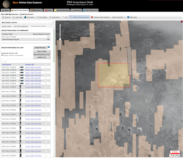
PDS Geosciences Node Mars Orbital Data Explorer (ODE).
I retrieved both the nadir image files and the areoid elevation.
It is also possible to download shapefiles of coverage footprints of various Mars satellite data and identify coverage of Souness GLF footprints in a more automated fashion.
The actual 6 band feature vector was
The software I used for this was Jo Wood's LandSerf. In his PhD thesis there is a good explanation of the various different types of topographic curvature. Unfortunately this is no longer easily accessible, except via the Internet Archive however the various types of curvature are also explained in this website forming part of an online textbook on Geospatial Analysis.
After processing in LandSerf I used gdal at the command-line to generate a layerstacked .kea file for each tile.
The longitudinal and cross-sectional curvatures are defined in the slope's own plane, i.e. the plane containing the slope vector with normal pointing in the aspect direction.
The longitudinal curvature is a measure of convexity/concavity of the slope, and cross-sectional curvature the rate of change of the slope vector, when considered in the slope's own reference frame (as opposed to plan curvature which considers the same from vertically above).
The 10 band layerstacks, which I didn't process further due to the processing time also included Mean curvature, plan curvature, profile curvature and Landserf feature classification.
Later on, in reprocessing the results after the dissertation I used the original aspect rather than the absolute aspect from N.
This is detailed in section 3.4.2 on pages 36-43 of the dissertation, or 43-52 of the tablet-optimised version I will try to recap it here.
The first step was to gather the data:
PDS Geosciences Node Mars Orbital Data Explorer (ODE).
I retrieved both the nadir image files and the areoid elevation.
It is also possible to download shapefiles of coverage footprints of various Mars satellite data and identify coverage of Souness GLF footprints in a more automated fashion.
The actual 6 band feature vector was
- Nadir image
- DTM elevation
- Slope (degrees)
- Aspect (in absolute degrees from north)
- Cross-sectional curvature
- Longitudinal curvature
The software I used for this was Jo Wood's LandSerf. In his PhD thesis there is a good explanation of the various different types of topographic curvature. Unfortunately this is no longer easily accessible, except via the Internet Archive however the various types of curvature are also explained in this website forming part of an online textbook on Geospatial Analysis.
After processing in LandSerf I used gdal at the command-line to generate a layerstacked .kea file for each tile.
The longitudinal and cross-sectional curvatures are defined in the slope's own plane, i.e. the plane containing the slope vector with normal pointing in the aspect direction.
The longitudinal curvature is a measure of convexity/concavity of the slope, and cross-sectional curvature the rate of change of the slope vector, when considered in the slope's own reference frame (as opposed to plan curvature which considers the same from vertically above).
The 10 band layerstacks, which I didn't process further due to the processing time also included Mean curvature, plan curvature, profile curvature and Landserf feature classification.
Later on, in reprocessing the results after the dissertation I used the original aspect rather than the absolute aspect from N.
 |
| TuiView screenshot of the h0037 HRSC DTM tile. I have coded red:slope, green:nadir image and blue:elevation. |

