Skrifennow
My blog, imported from Blogger and converted using Jekyll.
« Prev
1
2
3
4
5
6
7
8
9
10
11
12
13
14
15
16
17
18
19
20
21
22
23
24
25
26
27
28
29
30
31
32
33
34
35
36
37
38
39
40
41
42
43
44
45
46
47
Next »
Errors in the land cover assessment
Last time, I mentioned I was going to compare the ground control points to the classification.
Before I do that, I thought I'd compare the extents of classified woodland and water to OS VectorMap data.
I show the "commission error" - where the classification indicated something where OS VectorMap didn't, and "omission error" where OS VectorMap indicated something but the classification didn't.
Not all of the difference may be error in the classification, there may have been real change on the ground between the epoch of the image and the OS VectorMap data, or what is marked out as a woodland areas on VectorMap may include clearings, felled areas, or partially forested areas that were often classified as "Mosaic".
It is evident that the kind of first-order adjustment for seasonal change in NDVI etc. is not really adequate to prevent large shifts between classes, instead it is likely to be necessary to examine each landcover class in detail to see how its spectral properties change across the growing season.
Before I do that, I thought I'd compare the extents of classified woodland and water to OS VectorMap data.
I show the "commission error" - where the classification indicated something where OS VectorMap didn't, and "omission error" where OS VectorMap indicated something but the classification didn't.
Not all of the difference may be error in the classification, there may have been real change on the ground between the epoch of the image and the OS VectorMap data, or what is marked out as a woodland areas on VectorMap may include clearings, felled areas, or partially forested areas that were often classified as "Mosaic".
June 2006
 | ||
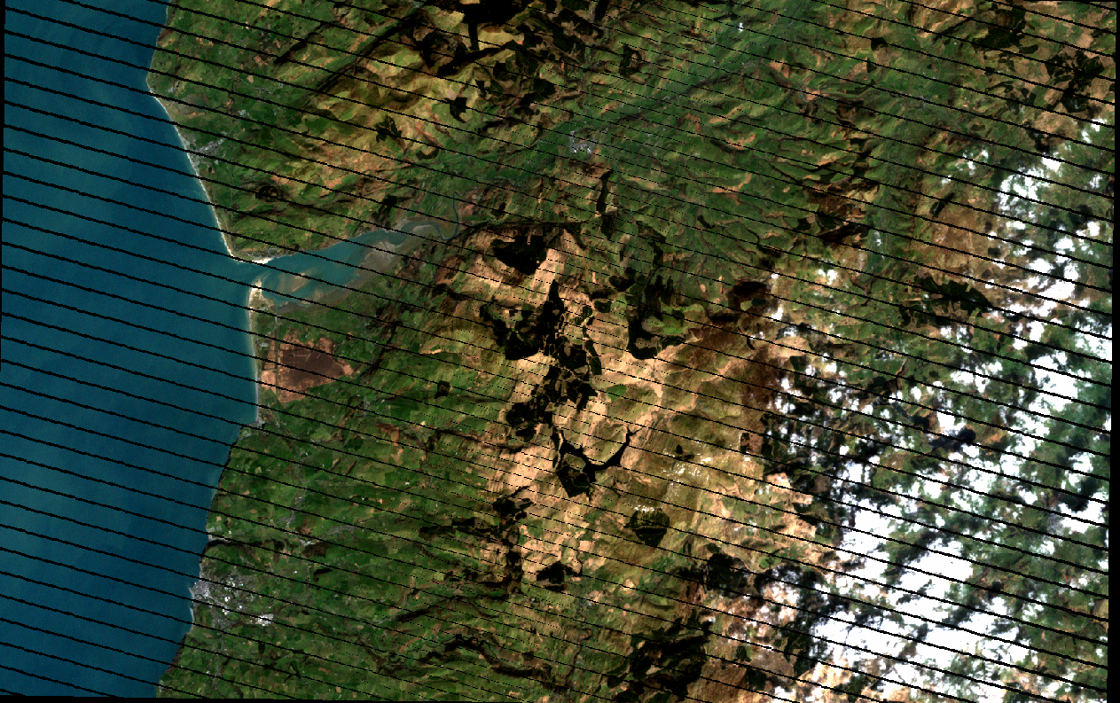
| RGB (9th June 2006) |
 | |
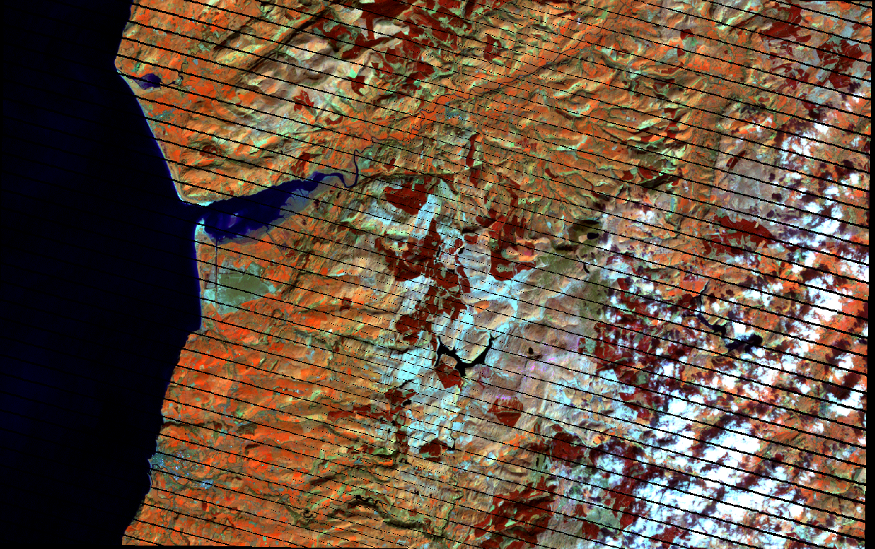
| NIR:SWIR1:Red 9th June 2006 |
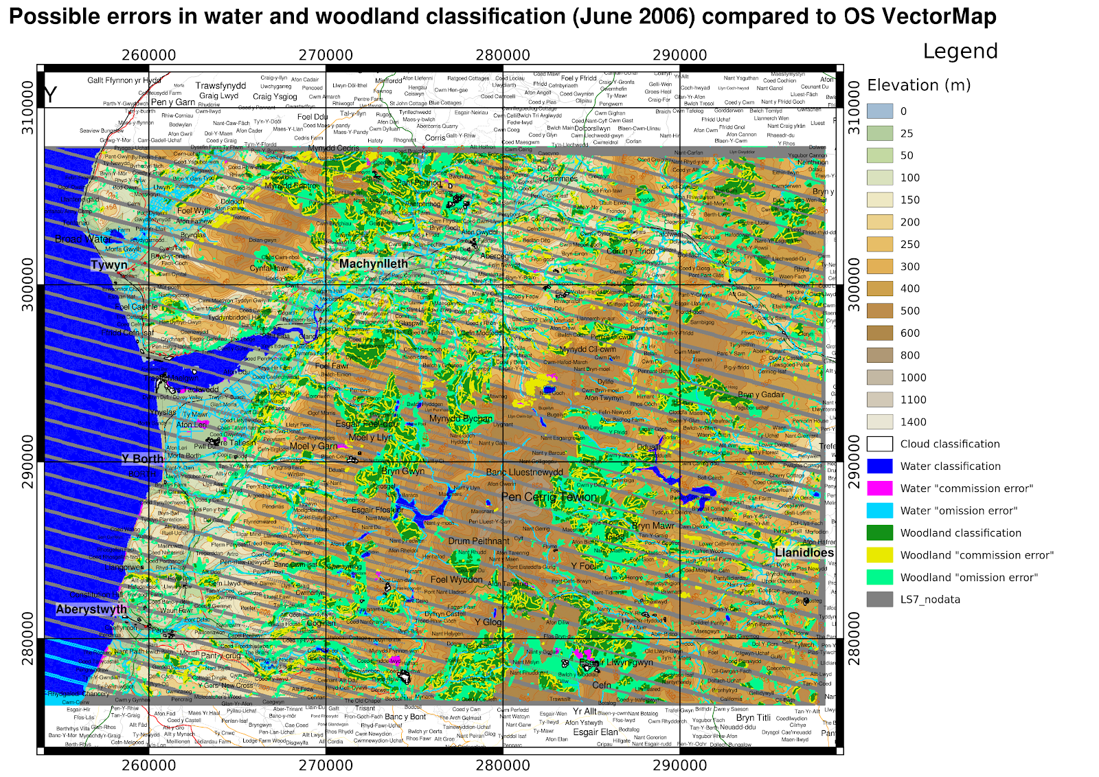 |
| large version There are a few areas of cloud shadow and other areas falsely classified as water. In addition there are some areas of cloud which may not be real. The woodland is generally underpredicted relative to OS VectorMap, the "omission error" areas are often classified as "Mosaic". |
March 2007
 |
| RGB 24th March 2007 |
 |
| NIR:SWIR1:Red 24th March 2007 |
 |
| large version This is perhaps the most accurate of the woodland classifications, though some of the woodland areas are missed particularly in the east of the image (where perhaps cloud is interfering to some extent) and is often classified as "mosaic". There are a few areas of bogusly classified water in topographic shadow areas |
September 2013
 |
| RGB (24th September 2013) |
 |
| NIR:SWIR1:Red |
 |
| large version Extensive areas of thin cloud appear in this image, woodland is overpredicted relative to OSVectorMap. It is likely that, late in the growing season, other vegetation has increased in NDVI and is perhaps masquerading as forest, or the subtle shadows of thin cloud are affecting the classification. Again some topographic shadowed areas are erroneously classed as water. |
Revisiting Land Cover assignment using Landsat
As part of one of the modules for my MSc in Remote Sensing and Planetary Science at Aberystwyth University, I did an assignment on land cover classification in Wales, using the LandSat satellites. I used data from Landsat 7 and Landsat 8.
The final maps from the assignment were somewhat basic, which I have revised below though I haven't changed the classification itself.
The classification scheme, was a rule-based one, where the rules were refined based on ground-control points taken using fieldwork.
I have put them into QGIS here, and added placename labels for context.
This is the first part of my revisiting this assignment. In future I will also say a little more about the ground control points from the fieldwork and how the results of the classification correspond to what was seen on the ground, and take this a little further than in the assignment report.
What would be really great, is to be able to automatically adjust a ruleset, rather than doing this by hand hard-coding into the scripts.
Landsat is a programme of Earth observation satellites launched by NASA and operated in cooperation with the US Geological Survey.
They have the capability to take data in several visible light bands, near infrared, short-wave infrared (this is longer wavelength than near-infrared but the common terminology in Earth Observation), and thermal infrared.
Landsat 8 has a slightly different range of wavelengths than Landsat 7, additionally having the 'Coastal' band in band 1 at a slightly shorter wavelength than the Blue band.
The area of study for the assignment was an area of mid-Wales including Aberystwth, and upland areas around Pumlumon.
We were set the images from Landsat 7 from March 2007 and June 2006 to work from, and I additionally used a Landsat 8 image from September 2013. Landsat 7 developer a scan line corrector fault. which resulted in black stripes where no data was collected.
The black no data stripes were ignored, in this classification, my view was to classify based on the data that exists, and perhaps use a nearest neighbour interpolation right at the end after classification if desired.
The various Landsat bands allow an overview of land cover types, based on the differing reflectance spectral properties of vegetation of various types, water, and non-vegetated surfaces. Living vegetation is strongly reflectant in the green and near-infrared, with dead vegetation reflecting more strongly at the longer 'short-wave infrared'.
Before classification, I first segmented to objects, for which I used the routine in the Python RSGISLib libraries:
In fact I segmented the image three different ways, in the assignment writeup I exclusively used the objects from segmenting the 24th March 2007 Landsat 7 image.
I made a kind of first order seasonal adjustment to the images, based on band averages in areas not classified as cloud or water. It was not entirely successful in creating a consistent classification as seen below.
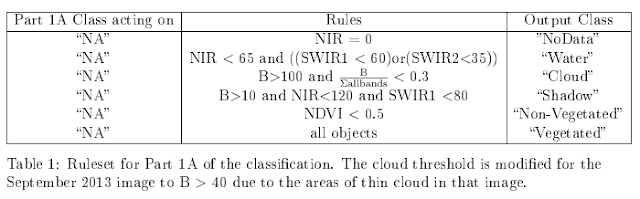
There are three stages to the process, first the Level 1A classification that delineates water (by low NIR and SWIR brightness), cloud (by high levels in the blue band), shadow (by thresholds in Blue, NIR, and SWIR1), and non-vegatation (by normalised differential vegatation index (NIR, R)).
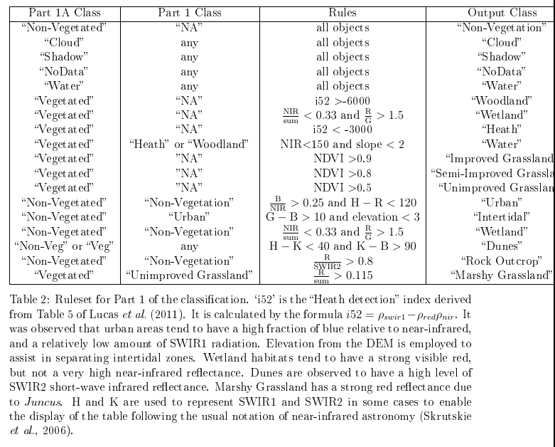
After this, in Level 1 split the vegetated areas into woodland, wetland, and heath, and grasslands into unimproved, semi-improved and improved by NDVI.
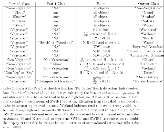
Level 2 classification splits woodland into broadleaf and coniferous, and wetlands into blanket bog and flush, and the upland vegetation further.
 For the other images, I made a first-order seasonal adjustment based on the average band values in non-water and non-cloud objects, effectively attempting to adjust back to the March image. I adjust the NDVI by half of its actual change to avoid overcorrection of the grassland classes, and the Lucas et al. 2011 heath detection index by a manually set value of +3000 in June and +5000 in September.
The final maps from the assignment were somewhat basic, which I have revised below though I haven't changed the classification itself.
The classification scheme, was a rule-based one, where the rules were refined based on ground-control points taken using fieldwork.
I have put them into QGIS here, and added placename labels for context.
This is the first part of my revisiting this assignment. In future I will also say a little more about the ground control points from the fieldwork and how the results of the classification correspond to what was seen on the ground, and take this a little further than in the assignment report.
What would be really great, is to be able to automatically adjust a ruleset, rather than doing this by hand hard-coding into the scripts.
The Data
Landsat is a programme of Earth observation satellites launched by NASA and operated in cooperation with the US Geological Survey.They have the capability to take data in several visible light bands, near infrared, short-wave infrared (this is longer wavelength than near-infrared but the common terminology in Earth Observation), and thermal infrared.
Landsat 8 has a slightly different range of wavelengths than Landsat 7, additionally having the 'Coastal' band in band 1 at a slightly shorter wavelength than the Blue band.
The area of study for the assignment was an area of mid-Wales including Aberystwth, and upland areas around Pumlumon.
We were set the images from Landsat 7 from March 2007 and June 2006 to work from, and I additionally used a Landsat 8 image from September 2013. Landsat 7 developer a scan line corrector fault. which resulted in black stripes where no data was collected.
The black no data stripes were ignored, in this classification, my view was to classify based on the data that exists, and perhaps use a nearest neighbour interpolation right at the end after classification if desired.
The various Landsat bands allow an overview of land cover types, based on the differing reflectance spectral properties of vegetation of various types, water, and non-vegetated surfaces. Living vegetation is strongly reflectant in the green and near-infrared, with dead vegetation reflecting more strongly at the longer 'short-wave infrared'.
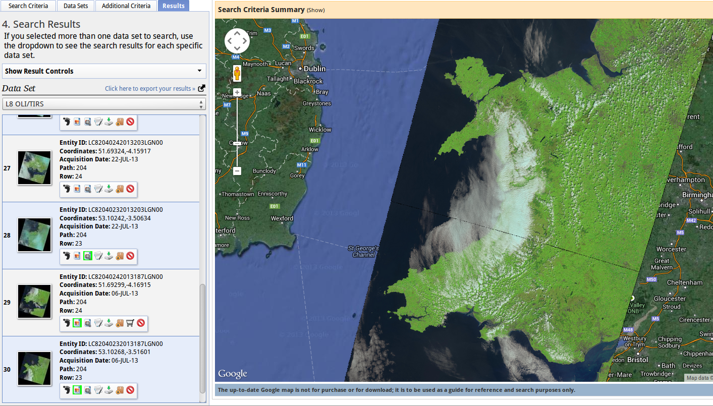 |
| A bank of cloud coincides with the area of study on 6th July 2013 |
 |
| Landsat 7: 9th June 2006, using Bands 3, 2 and 1 (red, green and blue) as RGB. |
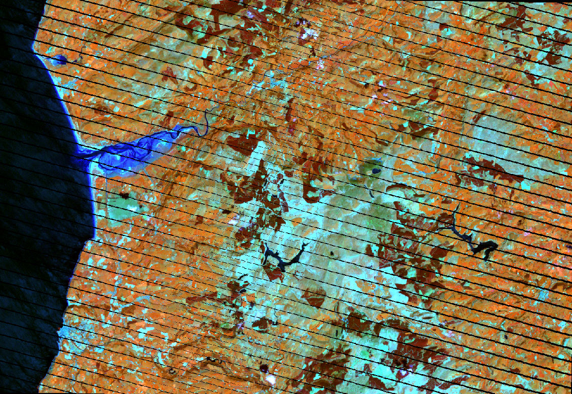 |
| Landsat 7: 9th June 2006, using Bands 4, 6 and 3 (NIR, SWIR1 and red) as RGB. |
 |
| Landsat 7: 24th March 2007, using bands 3, 2 and 1 (red, green, blue) as RGB. |
 |
| Landsat 7: 24th March 2007, using bands 4, 6 and 3 (NIR, SWIR1, red) as RGB. |
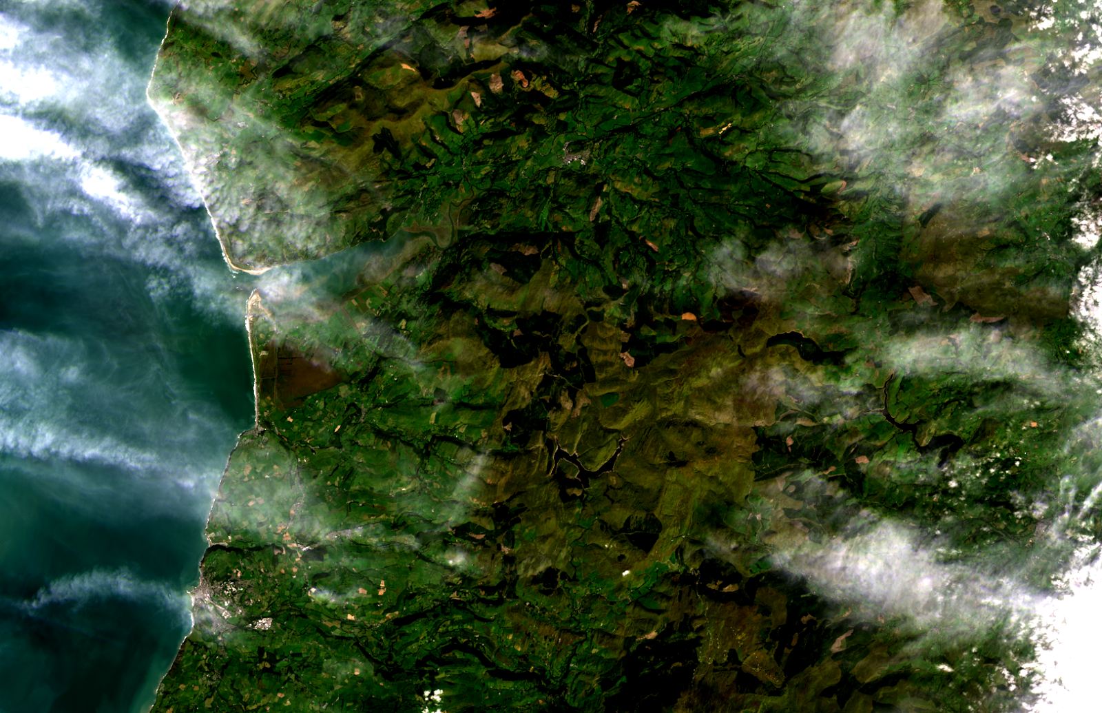 |
| Landsat 8: 24th September 2013, bands 4, 3 and 2 (red, green, blue) as RGB. |
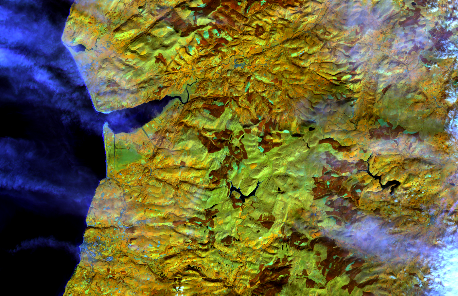 |
| Landsat 8: 24th September 2013, bands 5, 6 and 4 (NIR, SWIR1, red) as RGB. |
Classification
A rule based classification was used, inspired broadly speaking by the various Richard Lucas et al. papers: Lucas et al. 2007 Lucas et al. 2011.Before classification, I first segmented to objects, for which I used the routine in the Python RSGISLib libraries:
 |
| The 9th June 2006 image, segmented in RSGISLib using the runShepherdSegmentation method with 120 clusters and a minimum object size of 9 pixels (8100 sq.m), colourized randomly. |
I made a kind of first order seasonal adjustment to the images, based on band averages in areas not classified as cloud or water. It was not entirely successful in creating a consistent classification as seen below.
Ruleset
The ruleset I first developed on the March 2007 image because that had areas of cloud and therefore an opportunity to get the cloud masking right first.There are three stages to the process, first the Level 1A classification that delineates water (by low NIR and SWIR brightness), cloud (by high levels in the blue band), shadow (by thresholds in Blue, NIR, and SWIR1), and non-vegatation (by normalised differential vegatation index (NIR, R)).
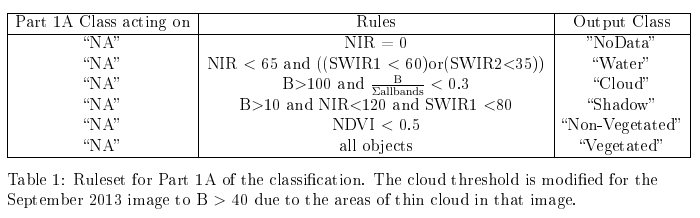
After this, in Level 1 split the vegetated areas into woodland, wetland, and heath, and grasslands into unimproved, semi-improved and improved by NDVI.
Level 2 classification splits woodland into broadleaf and coniferous, and wetlands into blanket bog and flush, and the upland vegetation further.

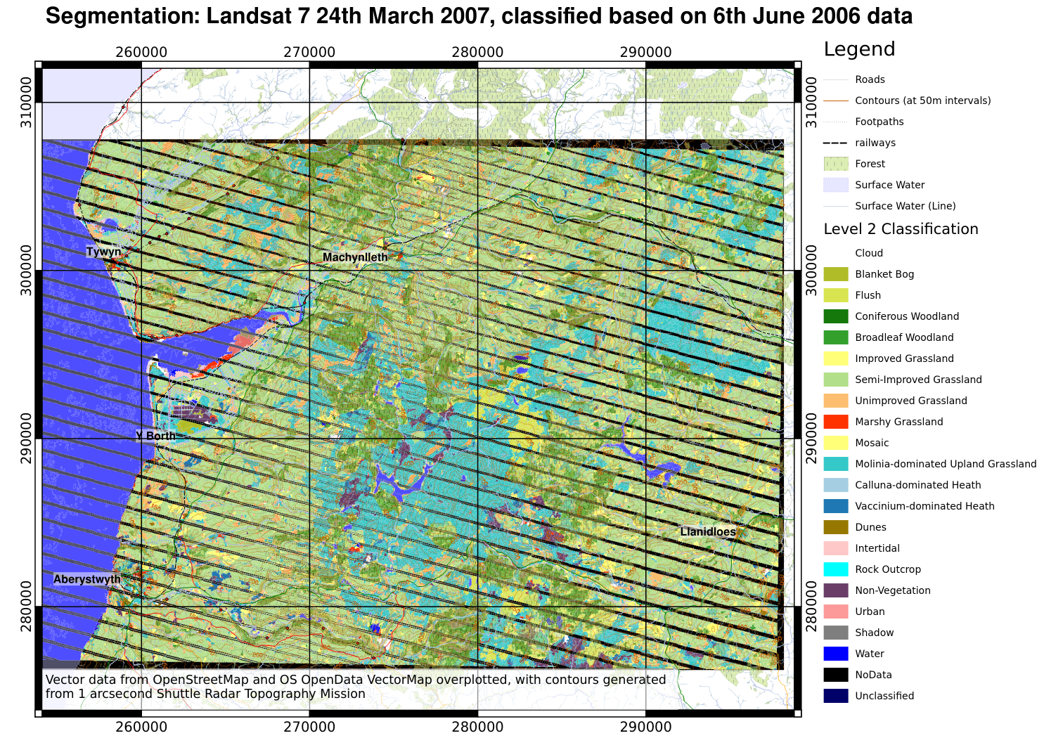
24th March 2007 segmentation
This was what I used in my report. There is a substantial area under cloud in the SE of the image. I have masked out areas that have No Data in one or both images. |
| The cloud areas are shown in the SE, generally woodland and water extents are well-recovered. large version |
 |
| Unfortunately some detail is lost in the uplands, and some areas are spuriously classified as non-vegetated. large version |
 |
| Modification of the cloud threshold was needed to mask out the extensive areas of thin cloud covering parts of the image. Some spurious water bodies are shown which are in face topographic shadow misclassified as water. large version |
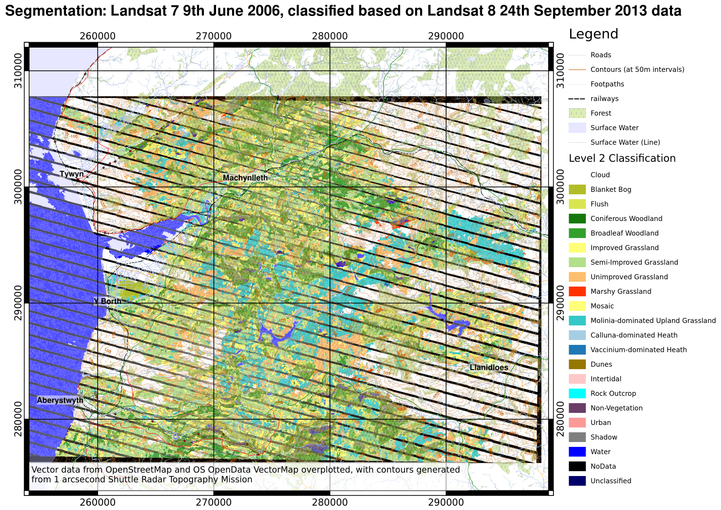
6th June 2006 segmentation
 |
| Again, the summer image does not differentiate the different type of upland vegetation well. The cloud shadow on Borth Bog is misclassified as water. large version |
 |
| The summer 2006 image is segmented and the spring 2007 data applied, there are some spurious classifications in the cloud shadow areas. large version |
 |
| The September 2013 data, again showing some spurious areas of water, and some errors around the margins of cloud. large version |
24th September 2013 segmentation
I only present the 24th September 2013 data, for this segmentation, due to problems that would be caused by the Landsat 7 no data stripes.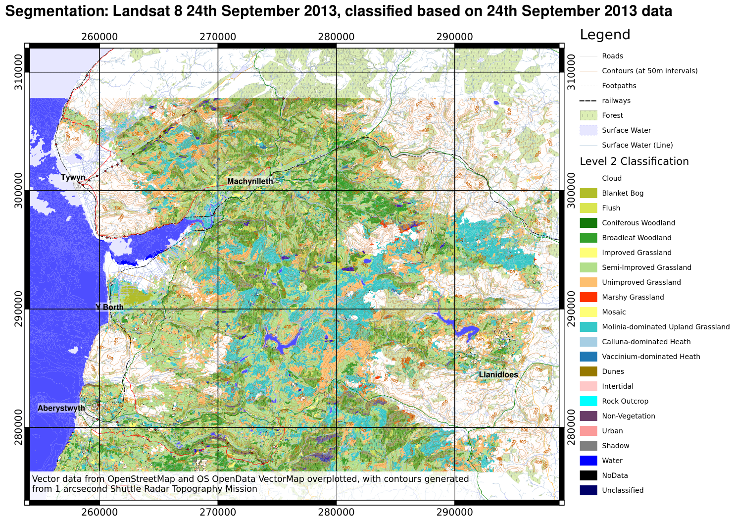 |
| Using the Landsat 8 image for segmentation avoids the stripes of no data, but delimiting the edges of thin cloud is difficult and may result in spurious classifications around the edges. The upland vegetation is not well delineated, with large areas assigned to 'unimproved grassland' or 'Molinia-dominated upland grassland'. large version |
It's #PlutoTime
Since 2003, NASA's New Horizons probe has been on its way to its Pluto flyby on 14th July 2015.
During this time it was demoted in status to dwarf planet by an International Astronomical Union committee.
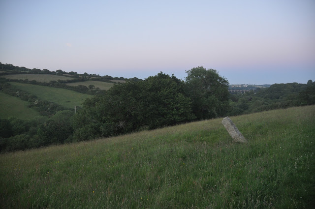
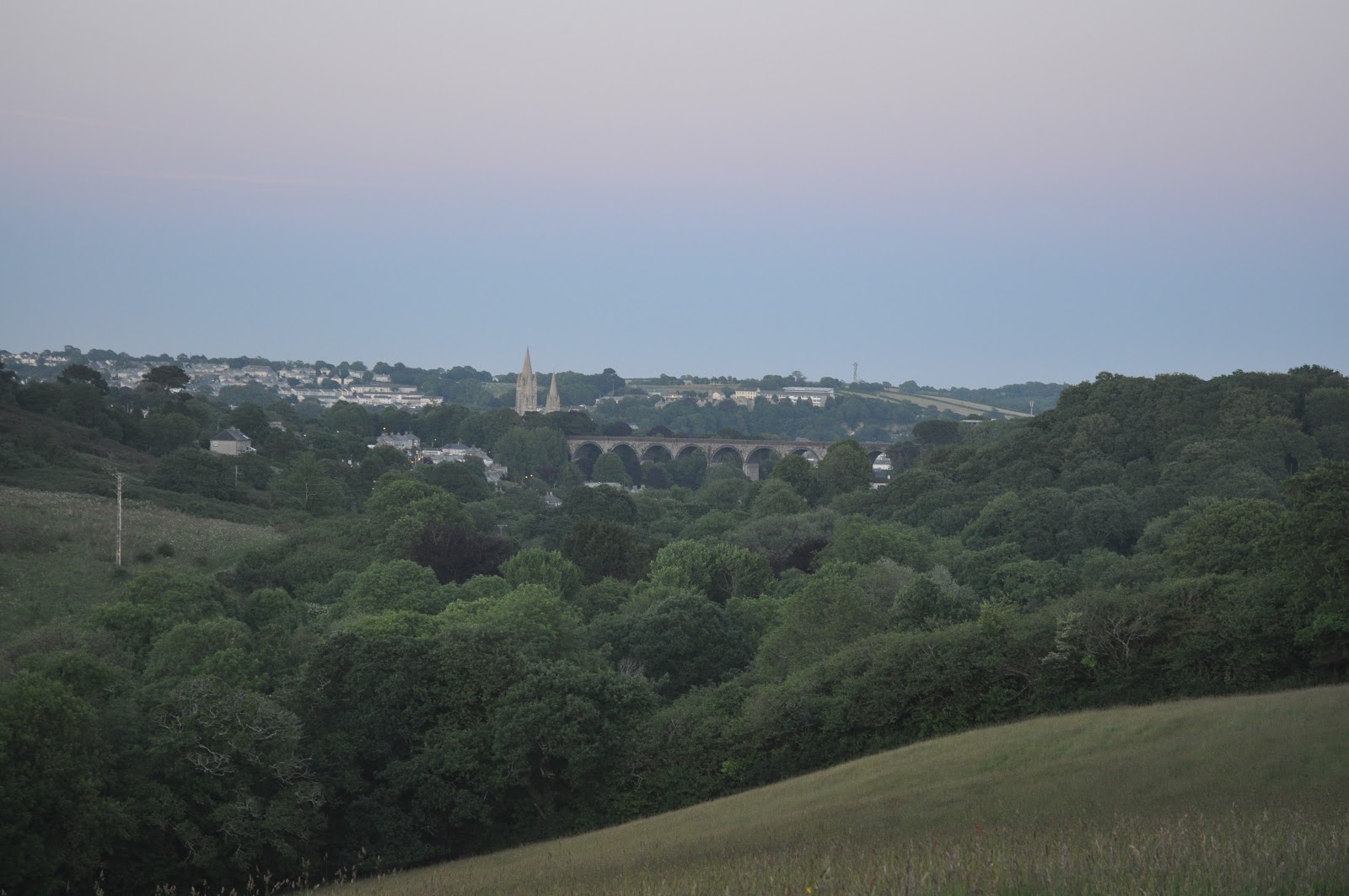
NASA is encouraging people to find out via the website here at what time of day (or rather after sunset) it will be as light as noon on Pluto, take a photograph and then share it using the hashtag #PlutoTime.
In Truro, Cornwall, it was 21:41 BST on 19th June.
So here are a few pictures of it:
During this time it was demoted in status to dwarf planet by an International Astronomical Union committee.
NASA is encouraging people to find out via the website here at what time of day (or rather after sunset) it will be as light as noon on Pluto, take a photograph and then share it using the hashtag #PlutoTime.
In Truro, Cornwall, it was 21:41 BST on 19th June.
So here are a few pictures of it:
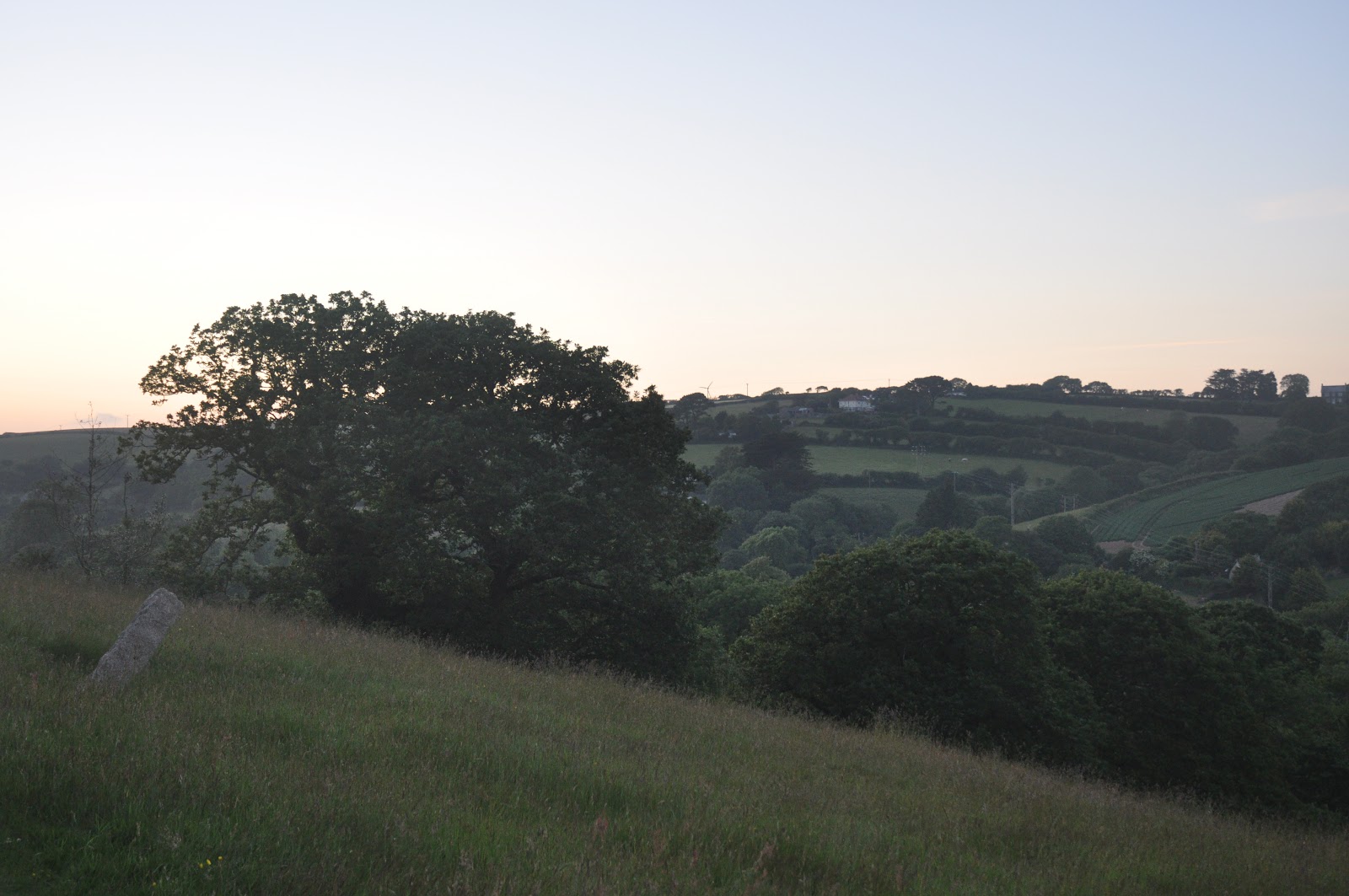 |
| Exposure 1/80 sec at ISO 640 |
 |

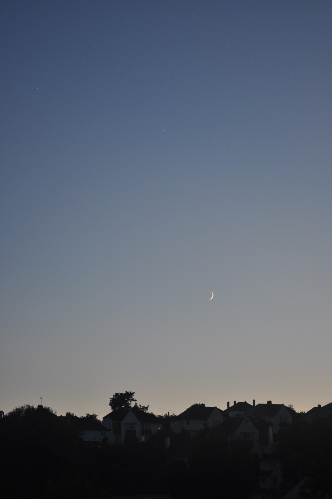 |
| About 15 minutes after #PlutoTime, imagine this is Charon and one of the small moons, though Charon is about 7 times larger in angular size seen from Pluto than the Earth's moon is from Earth. |
The Snows of Olympus, Part II
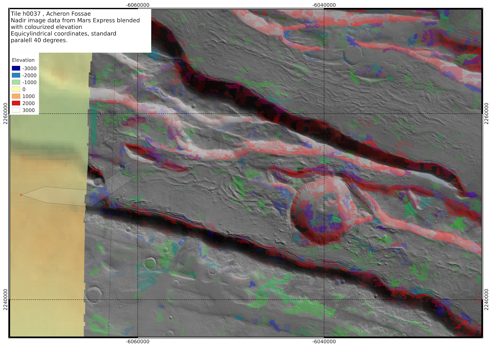
Here are some more maps from this same area, first focusing on the Acheron Fossae region of the h0037 tile.
I scale the elevation colourization locally:
Below, I zoom in on several areas containing several Souness catalogued GLFs, using either colourized elevation, or shading in polygons with ln(K_head), ln(K_ext), and ln(K_ctx) greater than 12, 10 or 10 respectively:
I scale the elevation colourization locally:
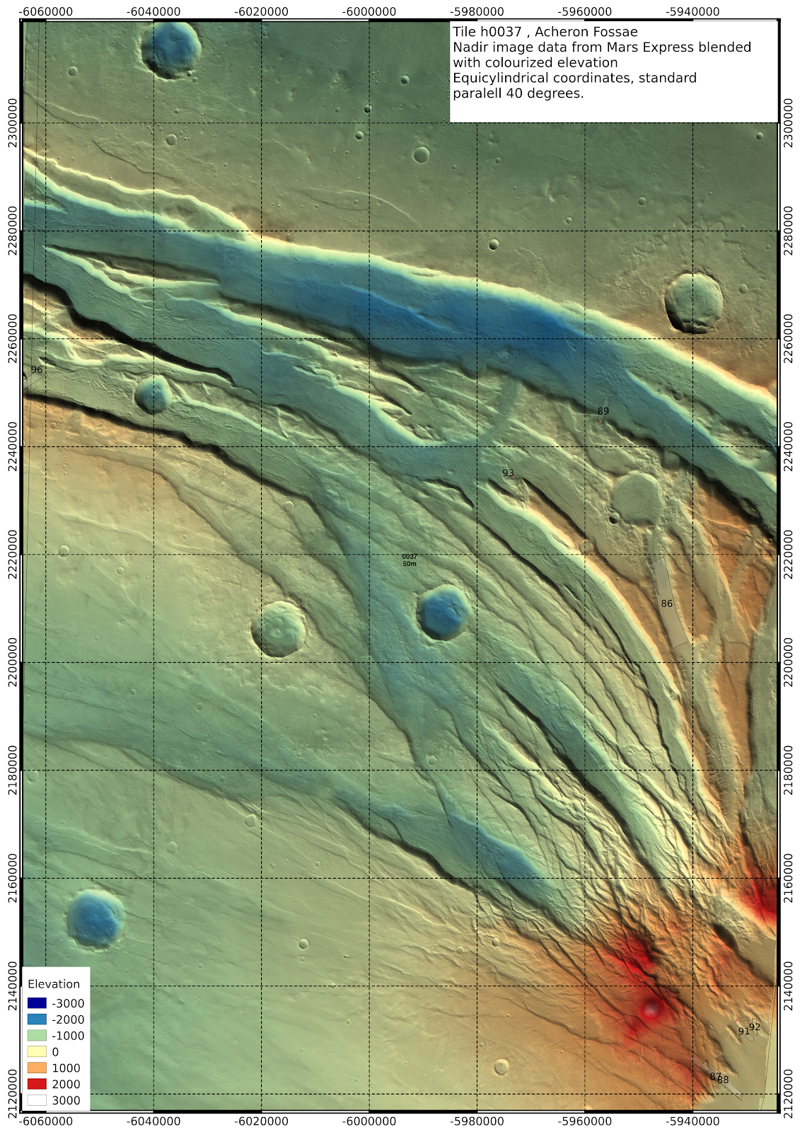 |
| large version (16MB) |
Below, I zoom in on several areas containing several Souness catalogued GLFs, using either colourized elevation, or shading in polygons with ln(K_head), ln(K_ext), and ln(K_ctx) greater than 12, 10 or 10 respectively:
 |
| large version |
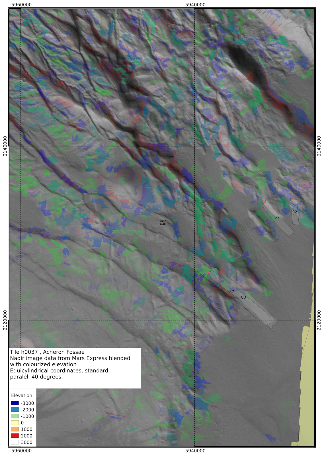 |
| large version of shaded polygons image |
 |
| large version |
 |
| large version |
 |
| large version |
 |
| large version |
 |
Souness catalogued GLF number 96 merits a closer examination to have a look what is going on with the polygon. |
 |
| large version |
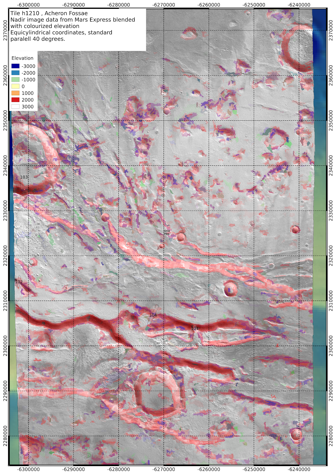
h1210
 |
| large version |
 |
| large version |
h1232
 |
| large version |
 |
| large version |
h5380
 | ||||||||
| It looks a little to me like the glacier filled the crater before it receded downwards (large version) |
 |
| large version |
The Snows of Olympus
The HRSC tile h0037 is a monster, it covers a vast area, the image file is 17568 x 144800 at 12.5m resolution and topography is 4391 x 36200 at 50m resolution. See also data product footprint at Mars ODE.
It covers an area including the summit of the vast Olympus Mons mountain, the largest on Mars and the largest volcano on any planet of the solar system.
There are a few Souness glacier-like forms in the north of the tile, the name 'Nix Olympia' dates back to the time of telescopic observations which perhaps mistook the brighter rocks of the Olympus Mons massif for snow.
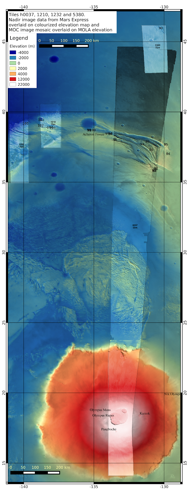
The Snows of Olympus is also the title of a book by Arthur C. Clarke which I have, containing some speculation about colonisation and terraforming Mars, along with some computer graphics renderings which were state of the art in the early 1990s of a Mars undergoing terraforming.
The above image shows the Olympus Mons Lobate Debris Apron, which is in fact thought to be glacial in origin, at the very high obliquity epochs in Mars' past, glacial activity is believed to have occured in the tropical mountain regions around the Tharsis bulge.
The Souness glacier like forms are concentrated to the north of the tile however, and in neighbouring tiles h1210, h1232 and h5280.
The above image showed up a significant issue with the dissertation. The Bayesian classifier used the nadir image data, as well as the digital terrain model and derived topographic values. However looking at the h5280 field at 130W 45N it is clear the scaling of the image brightness is separate for each tile, which means it doesn't mean much in the context of global statistics.
In the more detailed images below, an equicylindrical coordinate system is used with a standard parallel at 40 degrees of latitude.
Showing an area around 37N, 133W, in the Acheron Fossae region.

 h1210
h1210
larger version (22MB)


It covers an area including the summit of the vast Olympus Mons mountain, the largest on Mars and the largest volcano on any planet of the solar system.
There are a few Souness glacier-like forms in the north of the tile, the name 'Nix Olympia' dates back to the time of telescopic observations which perhaps mistook the brighter rocks of the Olympus Mons massif for snow.
Summary
larger version (12.7MB)The Snows of Olympus is also the title of a book by Arthur C. Clarke which I have, containing some speculation about colonisation and terraforming Mars, along with some computer graphics renderings which were state of the art in the early 1990s of a Mars undergoing terraforming.
The above image shows the Olympus Mons Lobate Debris Apron, which is in fact thought to be glacial in origin, at the very high obliquity epochs in Mars' past, glacial activity is believed to have occured in the tropical mountain regions around the Tharsis bulge.
The Souness glacier like forms are concentrated to the north of the tile however, and in neighbouring tiles h1210, h1232 and h5280.
The above image showed up a significant issue with the dissertation. The Bayesian classifier used the nadir image data, as well as the digital terrain model and derived topographic values. However looking at the h5280 field at 130W 45N it is clear the scaling of the image brightness is separate for each tile, which means it doesn't mean much in the context of global statistics.
In the more detailed images below, an equicylindrical coordinate system is used with a standard parallel at 40 degrees of latitude.
h0037
larger version (48MB)Showing an area around 37N, 133W, in the Acheron Fossae region.

h1210 and h1232
larger version (21MB)
larger version (22MB)

h5380
larger version (8MB)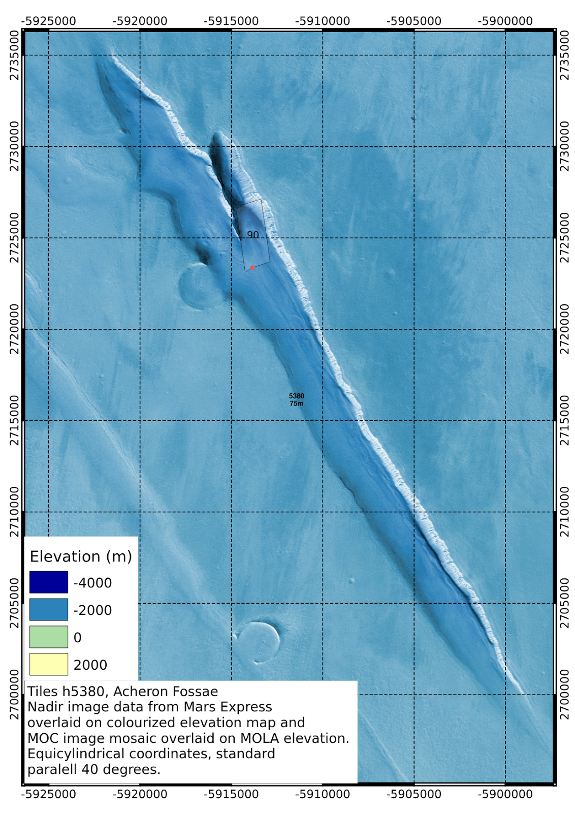
« Prev
1
2
3
4
5
6
7
8
9
10
11
12
13
14
15
16
17
18
19
20
21
22
23
24
25
26
27
28
29
30
31
32
33
34
35
36
37
38
39
40
41
42
43
44
45
46
47
Next »