Skrifennow
My blog, imported from Blogger and converted using Jekyll.
« Prev
1
2
3
4
5
6
7
8
9
10
11
12
13
14
15
16
17
18
19
20
21
22
23
24
25
26
27
28
29
30
31
32
33
34
35
36
37
38
39
40
41
42
43
44
45
46
47
Next »
The Bayesian classifier function in the dissertation - Part 3: Segmenting the layerstacked feature vector
In the previous post, I made an aside to mention what I did to create shapefiles of the Souness glacier-like-form extents.
Now I will mention the actual segmentation of the layerstacked feature vector.
The RSGISlib function that performs the segmentation is described on the RSGISlib website at www.rsgislib.org/rsgislib_segmentation.html.
I wrote a wrapper script around it to perform the segmentation itself, setting the smallest size of segments at 0.2 square kms. I calculate the number of pixels that is depending on the DTM resolution. This can be extracted via the gdalinfo command-line script.
One detail is that I added 9999 to all fields before using the segmentation, since the segmentation didn't work properly with negative values, which are encountered in Martian DTM data, and also in the DTM curvature fields.
There is a subtlely not mentioned in the above flowchart, is that I add the statistics from the original image file (i.e. without the +9999) to the clumps file from the segmentation to the RAT table.
In one version of RSGISLib, it didn't include the objectID in the raster attribute table, which I then added back in manually with a Python script.
The gdal_polygonize command takes the segment clumps file and makes it into shapefile polygons.
Now I will mention the actual segmentation of the layerstacked feature vector.
 |
| A figure from my dissertation showing the process of segmenting the layerstacked feature vector with RSGISlib, then using gdal_polygonize to convert this to a shapefile, and extracting the Raster Attribute Table as a .csv file, to which further processing can be done before rejoining the shapefile with it in QGIS. |
I wrote a wrapper script around it to perform the segmentation itself, setting the smallest size of segments at 0.2 square kms. I calculate the number of pixels that is depending on the DTM resolution. This can be extracted via the gdalinfo command-line script.
One detail is that I added 9999 to all fields before using the segmentation, since the segmentation didn't work properly with negative values, which are encountered in Martian DTM data, and also in the DTM curvature fields.
There is a subtlely not mentioned in the above flowchart, is that I add the statistics from the original image file (i.e. without the +9999) to the clumps file from the segmentation to the RAT table.
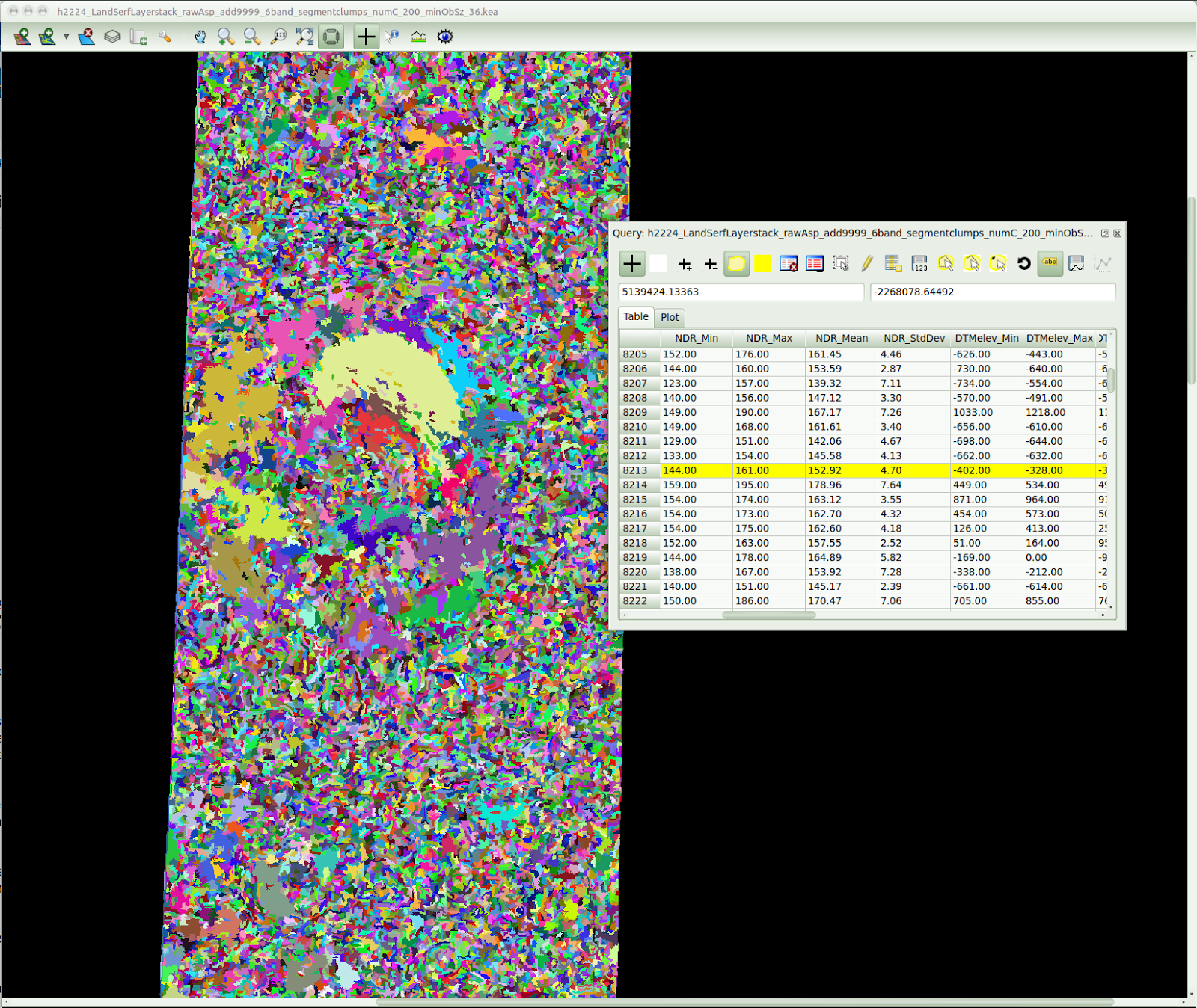 |
| Clumps file in TuiView for tile h2224 covering Greg crater, after the addition of the clump statistics to the RAT. |
In one version of RSGISLib, it didn't include the objectID in the raster attribute table, which I then added back in manually with a Python script.
The gdal_polygonize command takes the segment clumps file and makes it into shapefile polygons.
The Bayesian classifier function in the dissertation results - Part 2: getting the Souness catalogue into shapefile form
In order to focus on the areas of the Souness et al. 2012 glacier-like forms, I first needed to get the actual areas of interest as shapefiles.
I wrote some really not very good Python code to get the information from the Souness catalogue (a .csv exported from a spreadsheet which is available as a supplement from the paper itself) and then convert the coordinates of the GLF head, centre, terminus and left/right mid-channel from lat/long to an equicylindrical coordinate system with a standard parallel of 40°.
I have uploaded the code itself to my Bitbucket repository: bitbucket.org/davidtreth/marsglaciers
Later on in the process, these are intersected with the segmented DEM to find out zonal statistics on the subset of DEM segments that intersect with the Souness GLFs.
While digging around in the scripts I found that I in fact lost the script that actually did the zonal statistics for each DTM tile. I will have to rewrite it from a related one in the backups.
I used one script to loop through each of the HRSC fields and do zonal statistics with the GLF shapefiles. This produced a .csv file in the directory of each tile, and I used a further script to gather them all together into a single .csv file using the manually specified HRSC tile for each field.
Meanwhile, I recently adapted the script that made the Souness regions of interest, to make a series of intermediate areas along the midpoint of the glacier. :
I wrote some really not very good Python code to get the information from the Souness catalogue (a .csv exported from a spreadsheet which is available as a supplement from the paper itself) and then convert the coordinates of the GLF head, centre, terminus and left/right mid-channel from lat/long to an equicylindrical coordinate system with a standard parallel of 40°.
 |
| The Nilosyrtis Mensae area is fairly densely populated with Souness GLFs. |
I have uploaded the code itself to my Bitbucket repository: bitbucket.org/davidtreth/marsglaciers
 |
| A flowchart from my dissertation showing the usage of shapefiles of the Souness objects to create zonal statistics. |
While digging around in the scripts I found that I in fact lost the script that actually did the zonal statistics for each DTM tile. I will have to rewrite it from a related one in the backups.
I used one script to loop through each of the HRSC fields and do zonal statistics with the GLF shapefiles. This produced a .csv file in the directory of each tile, and I used a further script to gather them all together into a single .csv file using the manually specified HRSC tile for each field.
Meanwhile, I recently adapted the script that made the Souness regions of interest, to make a series of intermediate areas along the midpoint of the glacier. :
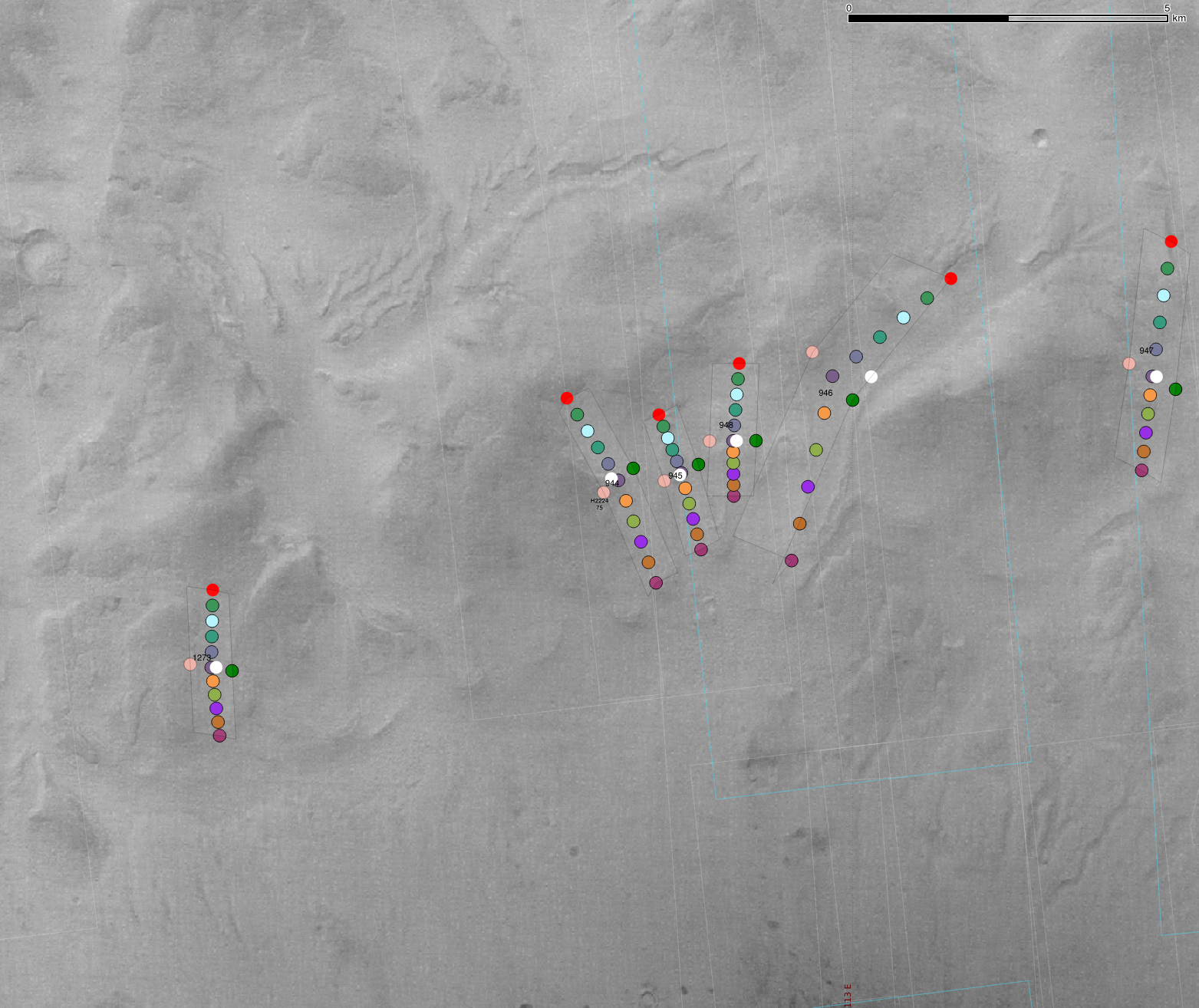 |
| A series of GLFs along the northern wall of Greg crater, with intermediate points along them, that could be useful for making approximate profiles, provided I can manage the rather opaque Python code involved in making the zonal statistics. |
The Bayesian classifier function in the dissertation results - Part 1: acquiring and preprocessing data
I have mentioned before a little about having a Bayesian classifier for the Martian terrain segments, which measures the similarity to the Martian terrain.
This is detailed in section 3.4.2 on pages 36-43 of the dissertation, or 43-52 of the tablet-optimised version I will try to recap it here.
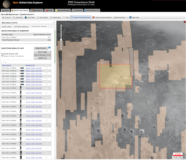
The first step was to gather the data:
I originally did this manually, inputting Souness GLF coorindinates manually into the web interface at PDS Geosciences Node Mars Orbital Data Explorer (ODE).
I retrieved both the nadir image files and the areoid elevation.
It is also possible to download shapefiles of coverage footprints of various Mars satellite data and identify coverage of Souness GLF footprints in a more automated fashion.
The actual 6 band feature vector was
The software I used for this was Jo Wood's LandSerf. In his PhD thesis there is a good explanation of the various different types of topographic curvature. Unfortunately this is no longer easily accessible, except via the Internet Archive however the various types of curvature are also explained in this website forming part of an online textbook on Geospatial Analysis.
After processing in LandSerf I used gdal at the command-line to generate a layerstacked .kea file for each tile.
The longitudinal and cross-sectional curvatures are defined in the slope's own plane, i.e. the plane containing the slope vector with normal pointing in the aspect direction.
The longitudinal curvature is a measure of convexity/concavity of the slope, and cross-sectional curvature the rate of change of the slope vector, when considered in the slope's own reference frame (as opposed to plan curvature which considers the same from vertically above).
The 10 band layerstacks, which I didn't process further due to the processing time also included Mean curvature, plan curvature, profile curvature and Landserf feature classification.
Later on, in reprocessing the results after the dissertation I used the original aspect rather than the absolute aspect from N.
This is detailed in section 3.4.2 on pages 36-43 of the dissertation, or 43-52 of the tablet-optimised version I will try to recap it here.
The first step was to gather the data:
 |
| Beginning with the tabulated Souness et al. 2012 objects, I identified and downloaded the relevant High Resolution and Stereo Camera DTM tiles, reprojected to a common equicylindrical cordinate system with a standard latitude of 40°, and then create derived topographic variables. |
I retrieved both the nadir image files and the areoid elevation.
It is also possible to download shapefiles of coverage footprints of various Mars satellite data and identify coverage of Souness GLF footprints in a more automated fashion.

The actual 6 band feature vector was
- Nadir image
- DTM elevation
- Slope (degrees)
- Aspect (in absolute degrees from north)
- Cross-sectional curvature
- Longitudinal curvature
The software I used for this was Jo Wood's LandSerf. In his PhD thesis there is a good explanation of the various different types of topographic curvature. Unfortunately this is no longer easily accessible, except via the Internet Archive however the various types of curvature are also explained in this website forming part of an online textbook on Geospatial Analysis.
After processing in LandSerf I used gdal at the command-line to generate a layerstacked .kea file for each tile.
The longitudinal and cross-sectional curvatures are defined in the slope's own plane, i.e. the plane containing the slope vector with normal pointing in the aspect direction.
The longitudinal curvature is a measure of convexity/concavity of the slope, and cross-sectional curvature the rate of change of the slope vector, when considered in the slope's own reference frame (as opposed to plan curvature which considers the same from vertically above).
The 10 band layerstacks, which I didn't process further due to the processing time also included Mean curvature, plan curvature, profile curvature and Landserf feature classification.
Later on, in reprocessing the results after the dissertation I used the original aspect rather than the absolute aspect from N.
 |
| TuiView screenshot of the h0037 HRSC DTM tile. I have coded red:slope, green:nadir image and blue:elevation. |
More zoomable images - on Mars this time
I previously shared my index to some of my posts about Martian glaciers.
I have produced zoomable images of the various parts of the Martian surface, with imagery from HRSC nadir images along with elevation.
Unfortunately, I have not been able to show the full resolution of these, because the method of tiling the 16384x16384 images I use as the basis of the work, using gdal2tiles.py and displaying using leaflet.js, involved a very large total number of files, and it seems my current web host at neocities.org has a maximum.
Nevertheless, the results can be seen at taklowkernewek.neocities.org/mars/hemispheres.html and taklowkernewek.neocities.org/mars/regions.html.
 |
| Sample screenshot from my website |
Update - it looks to me like even with only 4 zoomlevels, I have still managed to max out my number of files count. I am also in process of adding links to filtergraph.com where I have a number of scatter plots showing the Souness GLFs by region.
 |
| Numbers of Souness GLFs by region. |
 |
| An example of using Filtergraph to plot the various Souness GLFs in the Olympus Mons area. |
Using Leaflet.js for making my maps zoomable
I have come across the Javascript library Leaflet.JS which I have begun applying to my maps of Cornwall.
It may be used, in conjuction with Mapbox, to render OpenStreetMap in a number of styles, for example: link to taklowkernewek.neocities.org.
I have also made one of the versions of my cycling maps of Cornwall zoomable. This is simply done by rendering a 16384x16384px image of the map in QGIS, and then simply using Leaflet.js to make it zoomable, with the assistance of gdal2tiles.py to make the various 256px square tiles needed.
Link: taklowkernewek.neocities.org/mappys/leafletJStest/westcornwall.html
 |
| Follow link for zoomable version of this map, and also further maps of mid and east Cornwall. |
« Prev
1
2
3
4
5
6
7
8
9
10
11
12
13
14
15
16
17
18
19
20
21
22
23
24
25
26
27
28
29
30
31
32
33
34
35
36
37
38
39
40
41
42
43
44
45
46
47
Next »