Skrifennow
My blog, imported from Blogger and converted using Jekyll.
« Prev
1
2
3
4
5
6
7
8
9
10
11
12
13
14
15
16
17
18
19
20
21
22
23
24
25
26
27
28
29
30
31
32
33
34
35
36
37
38
39
40
41
42
43
44
45
46
47
Next »
Cornish identity in the 2011 census - part 2
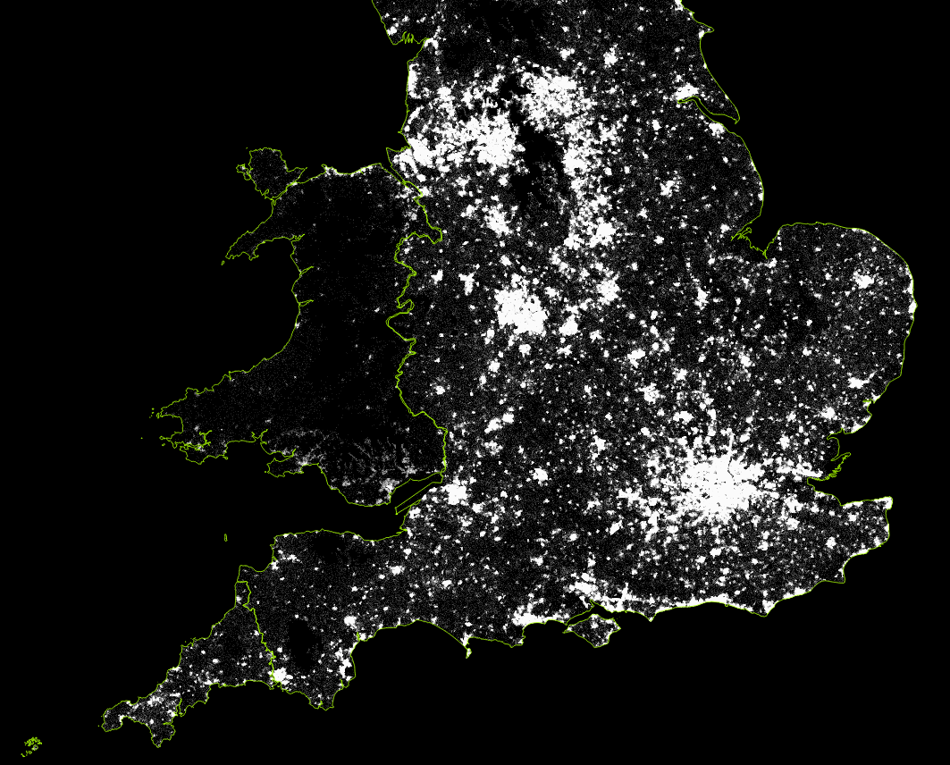
Here is a map showing people throughout Cornwall, England and Wales, who listed Cornish as their national identity:
These are random dots below 300m.
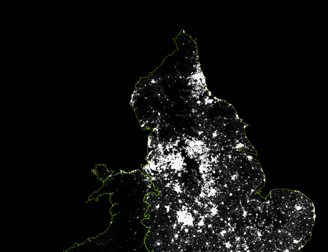
 Here is a map of people expressing Welsh identity:
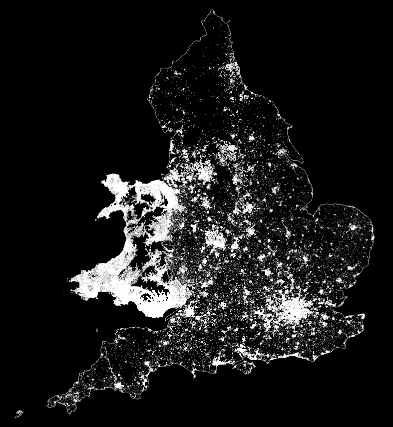 And English (reduced in number by a factor of 10):
These are random dots below 300m.
Cornish identity in the 2011 census
Here is a dot map representing all people in Cornwall declaring Cornish national identity in the 2011 census, generated using random points clipping the census output areas to the OS OpenData buildings layer.

As a heatmap, classifying by powers of 2:

As a heatmap, classifying by powers of 2:
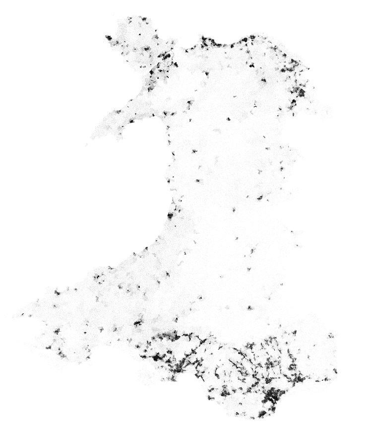
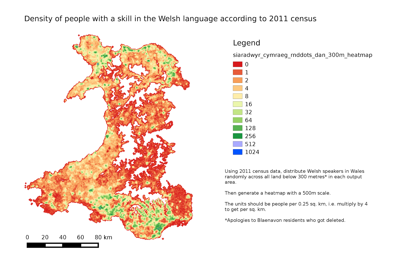
Speakers of the Welsh language according to 2011 census.
Much was written about a relatively small drop in the percentage of Welsh speakers in Wales as recorded by the 2011 census. I'm sure an astronomer wouldn't believe it was anything other than statistical noise if her data showed a 1% change from one survey to another....
Nevertheless, it is possible to visualise the data in a different way to the standard colorised maps you often see about these things.
One way is the restriction of the census output polygons to where buildings exist as the Datashine project did. However their website does not display statistics for Welsh language skills, since the detailed question was not asked to census respondents living outside Wales.
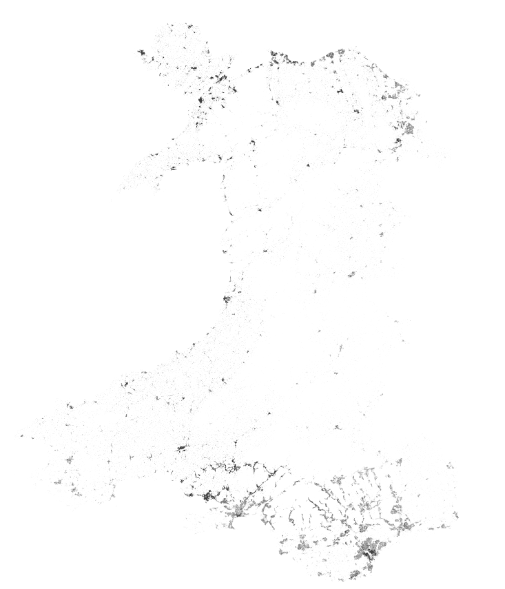
How about we use a QGIS plugin to give each Welsh speaker in Wales (or actually here, anyone claiming any skill in Welsh) a circular piece of land 50 metres wide, randomly located somewhere below 300 metres above sea level in his output census area polygon:

Nevertheless, it is possible to visualise the data in a different way to the standard colorised maps you often see about these things.
One way is the restriction of the census output polygons to where buildings exist as the Datashine project did. However their website does not display statistics for Welsh language skills, since the detailed question was not asked to census respondents living outside Wales.
How about we use a QGIS plugin to give each Welsh speaker in Wales (or actually here, anyone claiming any skill in Welsh) a circular piece of land 50 metres wide, randomly located somewhere below 300 metres above sea level in his output census area polygon:
So here we have the opposite problem to the issues with the typical visualisations with colourised choropleth maps where large but sparsely populated areas dominate visually,namely that denser areas are oversaturated at this scale.
It is also possible to take this random dot distribution and make it into a heatmap (click on the image for a larger version):
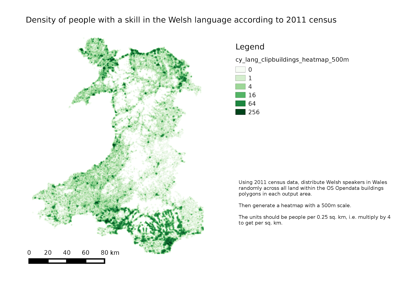
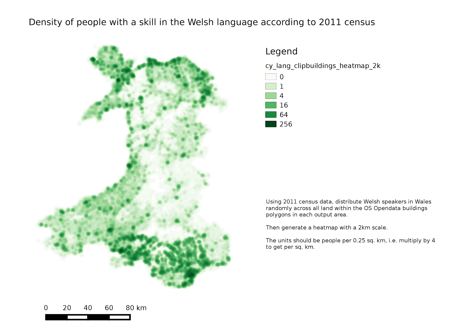
I also downloaded the OS OpenData buildings layer for the relevent grid squares covering Wales, and produced another dots distribution (this took QGIS some time).
This produces the following dot maps, giving each Welsh speaker 50 metre and 20 metre diameter circles of land respectively:
Heatmaps:
A little Python script to convert your Landsat scenes to KEA format
Downloading all this Mars data is starting to fill up my hard disks, so one thing I decided to do was compress all the various Landsat images I have.
Here is a Python script that will convert all GeoTIFF files in the current directory to the KEA format, and create a new header for each *MTL.txt Landsat header that exists in the directory to refer to the .kea files, for the use of a program such as ARCSI.
Download link (Dropbox)
# David Trethewey 20-06-2014
#
# convert all .tif or .TIF files
# in the current directory to .kea files
# using GDAL
# Does not delete any TIF files
#
# Assumptions:
# the TIF files are in the current directory
# that this script is being run from
# GDAL is available with KEA support
#
# Modifies any Landsat header *MTL.txt files so that
# arcsi.py works if you have compressed the
# band .TIF files to .kea
# Does not overwrite original header
#
# imports
import os.path
import sys
def replaceGTIFF_kea(inputtext):
outputtext = ""
for w in inputtext:
w = w.replace("GEOTIFF","KEA")
w = w.replace(".TIF",".kea")
# this line should be unnecessary since Landsat MTL files use capital letters
# but just in case you have one that doesn't
w = w.replace(".tif",".kea")
outputtext += w
return outputtext
# find all *.TIF files and *MTL.txt files in the current directory
directory = os.getcwd()
dirFileList = os.listdir(directory)
# print dirFileList
tifFileList = [f for f in dirFileList if ((f[-4:]=='.TIF')or(f[-4:]=='.tif'))]
MTLFileList = [f for f in dirFileList if (f[-7:]=='MTL.txt')]
#output format (GDAL code)
outFormat = 'KEA'
# run gdal_translate on all TIFs to convert to KEA
for t in tifFileList:
gdaltranscmd = "gdal_translate -of "+outFormat+" "+t+" "+t[:-4]+".kea"
print gdaltranscmd
os.system(gdaltranscmd)
# create a new header file referring to .kea files rather than .TIF
for m in MTLFileList:
inputtext = file(m).readlines()
outputtext = replaceGTIFF_kea(inputtext)
outputfilebase = m[:-4]
outputfile = outputfilebase + "_kea.txt"
out = file(outputfile,"w")
out.write(outputtext)
out.close()
Martian Crater "Greg" topographic and image segmentation
Here I have combined both topographic and image data from Mars Express High Resolution Stereo Camera, covering the area of the Martian crater Greg, which has been the subject of a recent study, allowing RSGISLib to segment a layerstack with elevation/slope/aspect and 4 image bands (BGRI).
The right-hand panel below has the blue image band in both blue and green channels, with elevation in the red channel.
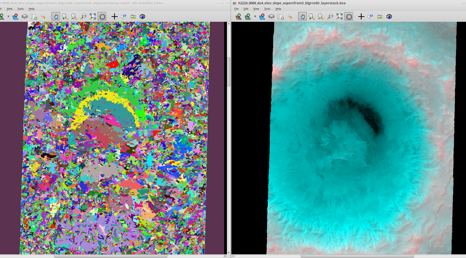 RSGISLib segmentation does seem to group certain areas together such as the crater floor, and gullies, but I have quite a long way to go before having a method to identify the glacier-like features automatically.
The right-hand panel below has the blue image band in both blue and green channels, with elevation in the red channel.
« Prev
1
2
3
4
5
6
7
8
9
10
11
12
13
14
15
16
17
18
19
20
21
22
23
24
25
26
27
28
29
30
31
32
33
34
35
36
37
38
39
40
41
42
43
44
45
46
47
Next »